Important Note: This article is part of the series in which TechReport.us discuss theory of Video Stream Matching.
2.7.2.1.1.2 – Step 2
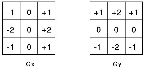
After smoothing the image and eliminating the noise, the next step is to find the edge strength by taking the gradient of the image. The Sobel operator performs a 2-D spatial gradient measurement on an image. Then, the approximate absolute gradient magnitude (edge strength) at each point can be found. The Sobel operator uses a pair of 3×3 convolution masks, one estimating the gradient in the x-direction (columns) and the other estimating the gradient in the y-direction (rows). They are shown below:

Figure 2.13 Vertical And Horizontal Masks
The magnitude, or EDGE STRENGTH, of the gradient is then approximated using the formula:
|G| = |Gx| + |Gy|
2.7.2.1.1.3 – Step 3
Finding the edge direction is trivial once the gradient in the x and y directions are known. However, you will generate an error whenever sumX is equal to zero. So in the code there has to be a restriction set whenever this takes place. Whenever the gradient in the x direction is equal to zero, the edge direction has to be equal to 90 degrees or 0 degrees, depending on what the value of the gradient in the y-direction is equal to. If GY has a value of zero, the edge direction will equal 0 degrees. Otherwise the edge direction will equal 90 degrees. The formula for finding the edge direction is just:
theta = invtan (Gy / Gx)
2.7.2.1.1.4 – Step 4
Once the edge direction is known, the next step is to relate the edge direction to a direction that can be traced in an image. So if the pixels of a 5×5 image are aligned as follows:
x x x
x x
x x x
x x
x x a
x x
x x x
x x
x x x
x x
Then, it can be seen by looking at pixel “a”, there are only four possible directions when describing the surrounding pixels – 0 degrees (in the horizontal direction), 45 degrees (along the positive diagonal), 90 degrees (in the vertical direction), or 135 degrees (along the negative diagonal). So now the edge orientation has to be resolved into one of these four directions depending on which direction it is closest to (e.g. if the orientation angle is found to be 3 degrees, make it zero degrees). Think of this as taking a semicircle and dividing it into 5 regions.
Therefore, any edge direction falling within the yellow range (0 to 22.5 & 157.5 to 180 degrees) is set to 0 degrees. Any edge direction falling in the green range (22.5 to 67.5 degrees) is set to 45 degrees. Any edge direction falling in the blue range (67.5 to 112.5 degrees) is set to 90 degrees. And finally, any edge direction falling within the red range (112.5 to 157.5 degrees) is set to 135 degrees.
2.7.2.1.1.5 – Step 5
After the edge
directions are known, non-maximum suppression now has to be applied.
Non-maximum suppression is used to trace along the edge in the edge
direction and suppress any pixel value (sets it equal to 0) that is
not considered to be an edge. This will give a thin line in the
output image.
2.7.2.1.1.6 – Step 6
Finally, hysteresis
is used as a means of eliminating streaking. Streaking is the
breaking up of an edge contour caused by the operator output
fluctuating above and below the threshold. If a single threshold, T1
is applied to an image, and an edge has an average strength equal to
T1, then due to noise, there will be instances where the edge dips
below the threshold. Equally it will also extend above the threshold
making an edge look like a dashed line. To avoid this, hysteresis
uses 2 thresholds, a high and a low. Any pixel in the image that has
a value greater than T1 is presumed to be an edge pixel, and is
marked as such immediately. Then, any pixels that are connected to
this edge pixel and that have a value greater than T2 are also
selected as edge pixels. If you think of following an edge, you need
a gradient of T2 to start but you don’t stop till you hit a gradient
below T1.
2.8 What is a Slope?
The color or gray-level slope is the maximum change between the intensity values of the center pixel and its neighboring pixels within a mask of pre determined size (such as 3×3). The slope direction is the direction of this maximum change.[6]
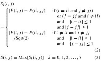
In general, the color or gray-level slope can be considered as a measure of the local intensity variation (change) within the image at a specific location, where as the slope direction indicates the direction of this intensity variation. In this study, we compute the slope magnitude an slope direction within a 3×3 mask. The computation of slope magnitude is done as follows:[6]

Figure 2.14 Slope Magnitude
where S(i, j)is the value of the slope magnitude at mask center location (i, j), P(i, j)is the pixel intensity/color value at the mask center location (i, j), and P(ii, jj)is the pixel value at a neighboring location within the mask.[6]
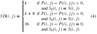
Since the result of the slope magnitude computation is a floating point number, the final result is converted into an integer and is scaled to lie between 0 and 255. The slope direction (SD)at location (i, j)is computed based on the value of k in Eq. (3) (when S(i, j) is determined) and the sign of [P(i, j)- P(ii, jj)], as[6]

Figure 2.15 Slope Direction
The slope feature, which includes the slope magnitudes and slope directions, represents local changes in pixel intensity/color values in the image. The total number of distinct components for the slope magnitude and slope direction feature sub vector is computed using the histograms of slope magnitude and slope direction values.


