
Important Note: This article is part of the series in which TechReport.us discuss theory of Video Stream Matching.
2.6 What is a Histogram?
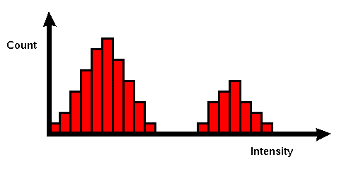
Figure 2.9 Intensity Histogram
In an image processing context, the histogram of an image normally refers to a histogram of the pixel intensity values. This histogram is a graph showing the number of pixels in an image at each different intensity value found in that image. For an 8-bit grayscale image there are 256 different possible intensities, and so the histogram will graphically display 256 numbers showing the distribution of pixels amongst those grayscale values. Histograms can also be taken of color images — either individual histograms of red, green and blue channels can be taken, or a 3-D histogram can be produced, with the three axes representing the red, blue and green channels, and brightness at each point representing the pixel count. The exact output from the operation depends upon the implementation — it may simply be a picture of the required histogram in a suitable image format, or it may be a data file of some sort representing the histogram statistics. [12, 13]
2.6.1 How It Works ?
The operation is very simple. The image is scanned in a single pass and a running count of the number of pixels found at each intensity value is kept. This is then used to construct a suitable histogram.
2.6.2 Guidelines for Use
Histograms have many uses. One of the more common is to decide what value of threshold to use when converting a grayscale image to a binary one by threshold. If the image is suitable for threshold then the histogram will be bi-modal — i.e. the pixel intensities will be clustered around two well-separated values. A suitable threshold for separating these two groups will be found somewhere in between the two peaks in the histogram. If the distribution is not like this then it is unlikely that a good segmentation can be produced by threshold.
2.7 What is an Edge?
Edge is the point in the image from where intensity level changes. This change is so much that it is notes able. So this is boundary between two intensity levels within same image.
Edges characterize boundaries and are therefore a problem of fundamental importance in image processing. Edges in images are areas with strong intensity contrasts – a jump in intensity from one pixel to the next. Edge detecting an image significantly reduces the amount of data and filters out useless information, while preserving the important structural properties in an image. [14]
2.7.1 How it Works ?
Based on this one-dimensional analysis, the theory can be carried over to two-dimensions as long as there is an accurate approximation to calculate the derivative of a two-dimensional image. The Sobel operator performs a 2-D spatial gradient measurement on an image. Typically it is used to find the approximate absolute gradient magnitude at each point in an input grayscale image.
The Sobel edge detector uses a pair of 3×3 convolution masks, one estimating the gradient in the x-direction (columns) and the other estimating the gradient in the y-direction (rows). A convolution mask is usually much smaller than the actual image. As a result, the mask is slid over the image, manipulating a square of pixels at a time.
The actual Sobel masks are shown below: [14]
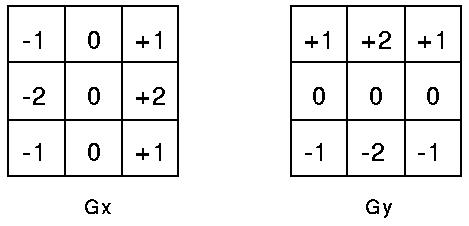
Figure 2.10 Sobal Masks
The magnitude of the gradient is then calculated using the formula[6]:
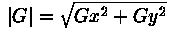
An approximate magnitude can be calculated using: [6]
|G| = |Gx| + |Gy|
2.7.2 Canny Edge Detection.
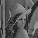
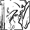
Figure 2.11 Canny Edges
The Canny edge detection algorithm is known to many as the optimal edge detector. Canny’s intentions were to enhance the many edge detectors already out at the time he started his work. He was very successful in achieving his goal and his ideas and methods can be found in his paper, “A Computational Approach to Edge Detection”. [16]
In his paper, he followed a list of criteria to improve current methods of edge detection. The first and most obvious is low error rate. It is important that edges occurring in images should not be missed and that there be NO responses to non-edges. [6]
The second criterion is that the edge points be well localized. In other words, the distance between the edge pixels as found by the detector and the actual edge is to be at a minimum.
A third criterion is to have only one response to a single edge. This was implemented because the first 2 were not substantial enough to completely eliminate the possibility of multiple responses to an edge.
Based on these criteria, the canny edge detector first smoothes the image to eliminate and noise. It then finds the image gradient to highlight regions with high spatial derivatives. The algorithm then tracks along these regions and suppresses any pixel that is not at the maximum (non maximum suppression).
The gradient array is now further reduced by hysteresis. Hysteresis is used to track along the remaining pixels that have not been suppressed. Hysteresis uses two thresholds and if the magnitude is below the first threshold, it is set to zero (made a non edge ). If the magnitude is above the high threshold, it is made an edge. And if the magnitude is between the 2 thresholds, then it is set to zero unless there is a path from this pixel to a pixel with a gradient above T2.
2.7.2.1 Guide Lines for Use
In order to implement
the canny edge detector algorithm, a series of steps must be
followed. The first step is to filter out any noise in the original
image before trying to locate and detect any edges. And because the
Gaussian filter can be computed using a simple mask, it is used
exclusively in the Canny algorithm.
2.7.2.1.1 Six Steps For Canny Algorithm
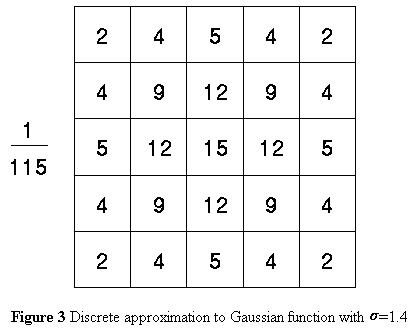
2.7.2.1.1.1 – Step 1
Once a suitable mask has been calculated, the Gaussian smoothing can be performed using standard convolution methods. A convolution mask is usually much smaller than the actual image. As a result, the mask is slid over the image, manipulating a square of pixels at a time. The larger the width of the Gaussian mask, the lower is the detector’s sensitivity to noise. The localization error in the detected edges also increases slightly as the Gaussian width is increased. The Gaussian mask used in my implementation is shown below.