

Important Note: This article is part of the series in which TechReport.us discuss theory of Video Stream Matching.
3.2.2.2.1 – How the KS Test Works?
In looking at a list of numbers, for example, the controlB group results from the second example:
controlB={1.26, 0.34, 0.70, 1.75, 50.57, 1.55, 0.08, 0.42, 0.50, 3.20, 0.15, 0.49, 0.95, 0.24, 1.37, 0.17, 6.98, 0.10, 0.94, 0.38}
It is hard to see the general situation. Thus descriptive statistics were developed to reduce the list of all the data items to a few simpler numbers. Thus perhaps better interpret data set from the following:
Mean=3.61
Median=0.60
High=50.6
Low=0.08
Standard Deviation = 11.2
We can see from this that something is abnormal. For normally distributed data you should expect about 15% of the data to lie more than 1 standard deviation below the mean (i.e., below 3.61-11.2=-7.59), but no data are that small, in fact no datum is even negative. Similarly only about 2% of the data should be more than 2 standard deviations above the mean (i.e., above 3.61+2×11.2=26.01), but in fact one data-point (50.57) way beyond that (hence an “outlier”).
3.2.2.2.2 – Cumulative Fraction Function & Empirical Distribution Function
The cumulative fraction function and the empirical distribution function are two names for the same thing: a graphical display of how the data is distributed. If you sort the controlB dataset from small to large you get: [25]
sorted controlB={0.08, 0.10, 0.15, 0.17, 0.24, 0.34, 0.38, 0.42, 0.49, 0.50, 0.70, 0.94, 0.95, 1.26, 1.37, 1.55, 1.75, 3.20, 6.98, 50.57}
Evidently no data lies strictly below 0.08, 5%=.05=1/20 of the data is strictly smaller that 0.10, 10%=.10=2/20 of the data is strictly smaller than 0.15, 15%=.15=3/20 of the data is strictly smaller than 0.17… There are 17 data points smaller than , and hence we’d say that the cumulative fraction of the data smaller than is .85=17/20. For any number x, the cumulative fraction is the fraction of the data that is strictly smaller than x. Below is the plot of the cumulative fraction for our control data. Each step in the plot corresponds to a data-point.
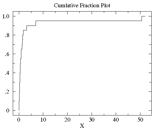
You can see with a glance that the vast majority of the data is scrunched into a small fraction of the plot on the far left. This is a sign of a non-normal distribution of the data.
In order to better see the data distribution, it would be nice to scale the x-axis differently, using more space to display small x data points. Since all the data are positive you can use a “log” scale. (Since the logarithm of negative numbers and even zero is undefined, it is not possible to use a log scale if any of the data are zero or negative.)
Since many measured quantities are guaranteed positive (the width of a leaf, the weight of the mouse, [H+]) log scales are common in science. Here is the result of using a log scale:
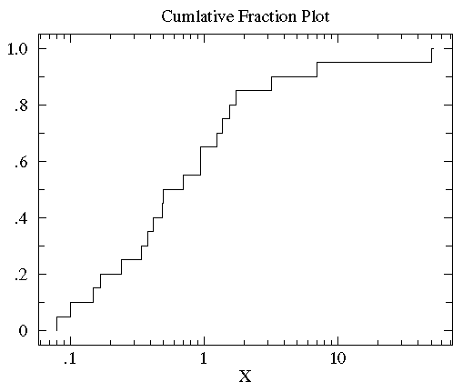
You can now see that the median (the point that divides the data set evenly into two: half above the median, half below the median) is a bit below 1.
Now plot the cumulative fraction of the treatment group on the same graph as we plotted the control cumulative fraction. (Use a dashed line to display the treatment group so distinguish it from the control group.)
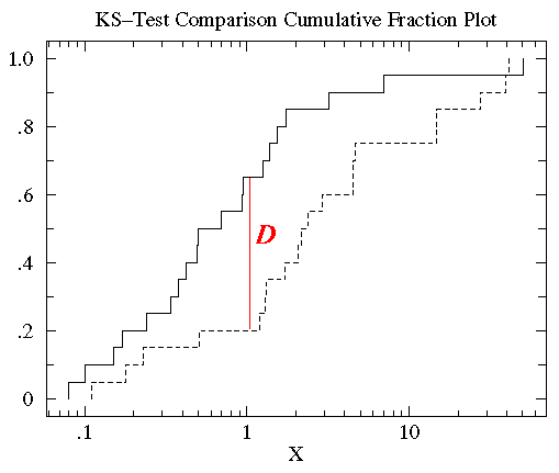
Figure 3.3
You can see that the control and treatment datasets span much the same range of values (from about .1 to about 50). But for most any x value, the fraction of the treatment group that is strictly less than x is clearly less than the fraction of the control group that is less than x.
That is, by-and-in-large the treatment values are larger than the control values for the same cumulative fraction. For example, the median (cumulative fraction =.5) for the control is clearly less than one whereas the median for the treatment is more than 1.
The KS-test uses the maximum vertical deviation between the two curves as the statistic D. In this case the maximum deviation occurs near x=1 and has D=.45. (The fraction of the treatment group that is less then one is 0.2 (4 out of the 20 values); the fraction of the control group that is less than one is 0.65 (13 out of the 20 values). Thus the maximum difference in cumulative fraction is D=.45.)