Important Note: This article is part of the series in which TechReport.us discuss theory of Video Stream Matching.
3.3.2 – Edge Features Extraction
Edge feature is consists on two elements.[6]
- Edge Map
- Edge Direction
3.3.2.1 – Edge Map
This is the feature which provides the map of edge in the image. This is the actually map of main element of the image. Usually each clip has unique element so this represent by that map.
To calculate it same procedure adopt as expressed in the “Canny Edge Detector Algorithm” in Chapter 2. Same six steps are taken.
Mathematically:
Number of elements of Edge Feature Sub Vector is same to the number of pixels of image.
R = Rows of Image
C = Column of Image
EM_Vec = R x C
3.3.2.2 – Edge Direction
This is the feature which is change in the usual algorithm of “Canny Edge Detector Algorithm”. [6]
Total direction is divided in to four directions. Angles from 0 degree to 180 degree divided into four parts.
Four directions are determined, in which the direction indicator is set to 1 for with value between 0 and 22.5 as well as between 157.5 and 180, set to 2 for with value between 22.5 and 67.5, set to 3 for with value between 67.5 and 112.5, set to 4 for with value between 122.5 and 157.5.
Directions are calculated using Gaussian Values as define in chapter 2.
Now convert whole image into tiles which are not over lapping. As image must be in the power of two. Tile’s size is according to rules into the power of two. So in next step calculate each angle occurred number of times in each tile and make its data. So each tile gives 4 values.
For better result each tile’s values are multiplying by a column matrix which has values from 1 to 4. As this technique apply in histogram.
This data is arranged in similar fashion as in histogram like each tile’s data is in one column. So number of tiles is same to number of column. Total values are get from this procedure is equal to number of tiles multiplying by 4.
NW = Number of Tiles
R = Rows of image
C = Columns of Image
16 x 16 = Size of each tile.
NW = ( R x C ) / (16×16)
EA_Vec = Number of Elements per image.
EA_Vec = NW * 4
3.3.3 – Slope Features Extraction
In Gray-Level Slope Magnitude and Slope Direction gray-level slope is the maximum change between the intensity values of the center pixel and its neighboring pixels within a mask of predetermined size (suchas3×3). The slope direction is the direction of this maximum change. Slope signs are the signs of values which got after maximum change direction calculation values. [6]
Total three kinds of features are calculated.
- Slope Magnitude
- Slope Direction
- Slope Signs
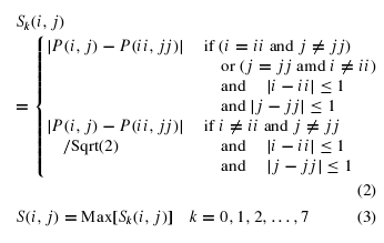
3.3.3.1 – Slope Magnitude

Figure 3.4
S ( i, j ) is the values of slope magnitude and these are calculated according to above mathematical description.
Total Sub _ Feature Vector is:
R = Rows of Image
C = Columns of Image
SM_Vec = Total number of elements per Image for slope Magnitude
SM_Vec = R x C
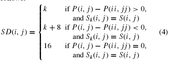
3.3.3.2 – Slope Direction

Figure 3.5
Slope direction is calculated as above mathematical description. Where it is step after the slope magnitude. SD ( i, j ) is the matrix of same size as slope magnitude.
So Mathematically:
SD_Vec = Total number of elements per Image for Slope Direction
SD_Vec = SM_Vec
3.3.3.3 – Slope Signs
When slope magnitude is calculating then values got in the form of
- >0
- <0
- =0
So using these values is use full for classification. So with pixel neglect the absolute values calculation technique and got the sign and store them then as in histogram apply tiles here also and within each tile calculate the number of positive values number of negative values and number of zero values. Arrange them into array form.
Mathematically:
NW = Number of Tiles per image
R = Rows of image
C = Columns of Image
NW = ( R x C ) / (16×16)
SS_Vec = Total number of elements per Image for Slope Signs
SS_Vec = NW * 3


