

Important Note: This article is part of the series in which TechReport.us discuss theory of Video Stream Matching.
2.2 – Image Processing
Image processing is a Computer imaging application involving a human being in the visual loop. It consists of following major fields:
- Image restoration
- Image enhancement
- Image compression
Image processing is the science of manipulating a picture. Image processing is often confused with computer graphics. Computer graphics and image processing are companion technologies. Although there are many common concepts between image processing and computer graphics, they are two separate studies.
Computer graphics is the generation of synthetic images. Image processing is the manipulation of images that have already been captured or generated. Computer graphics works with 2-dimensional and 3-dimensional objects. Image processing typically deals with but is not limited to 2-dimensional data. Applications in the medical diagnostic industry perform image processing on 3-dimensional data. With the emergence of certain technologies such as volume visualization and morphing, the dividing line between computer graphics and image processing is getting hazier.
2.3 – Some Basic Relationships Between Pixels
We consider several important relationships between pixels in a digital image. We represent an image by a 2D function f(x, y). When referring in this section to a particular pixel, we use lowercase letters, such as p and q.[1, 2]
2.3.1 – Neighbors of Pixel
A pixel p at coordinates (x, y) has four horizontal and vertical neighbors whose coordinates are given by
(x + 1, y), (x – 1, y), (x, y + 1), (x, y – 1)
This set of pixels, called the 4-neighbors of p, is denoted by N4 (p). Each pixel is a unit distance from (x, y), and some of the neighbors of p lie outside the digital image if (x, y) is on the border of the image.
The four diagonal neighbors of p have coordinates
(x + 1, y + 1), (x + 1, y – 1), (x – 1, y + 1), (x – 1, y – 1)
and are denoted by ND(p). These points, together with the 4-neighbors, are called the 8-neighbors of p, denoted by N8(p). As before, some of the points in ND(p) and N8(p) fall outside the image if (x, y) is on the border of the image.
2.3.2 – Adjacency, Connectivity, Regions and Boundaries
Connectivity between pixels is a fundamental concept that simplifies the definition of numerous digital image concepts, such as regions and boundaries. To establish if two pixels are connected, it must be determined if they are neighbors and if their gray levels satisfy a specified criterion of similarity (say, if their gray levels are equal). For instance, in a binary image with values 0 and 1, two pixels may be 4-neighbors, but they are said to be connected only if they have the same values. Let V be the set of gray-level values used to define adjacency. In a binary image, V = {1} if we are referring to adjacency of pixels with values 1.
In a gray scale image, the idea is the same, but set V typically contains more elements. For example, in the adjacency of pixels with a range of possible gray-level values 0 to 255, set V could be any subset of these 256 values. We consider three types of adjacency:[2]
- 4-adjacency. Two pixels p and q with values from V are 4-adjacent if q is in the set N4(p).
- 8-adjacency. Two pixels p and q with values from V are 8-adjacent if q is in the set N8(p).
- m-adjacency(mixed adjacency). Two pixels p and q with values from V are m-adjacent if q is in N4(p), or q is in ND(p) and the set N4(p)∩N4(q) has no pixels whose values are from V.
Mixed adjacency is a modification of 8-adjacency. It is introduced to eliminate the ambiguities that often arise when 8-adjacency is used. For example, consider the pixel arrangement shown in Fig. 2.1(a) for V = {1}.
The three pixels at the top of Fig. 2.1(b) show multiple (ambiguous) 8-adjacency, as indicated by the dashed lines. This ambiguity is removed by using m-adjacency, as shown in Fig 2.1(c). Two image subsets S1 and S2 are adjacent if some pixel in S1 is adjacent to some pixel in S2. It is understood here and in the following definitions that adjacent means 4-, 8-, or m-adjacent.
| 0 1 1 0 1 0 0 0 1 | 0 1 1 0 1 0 0 0 1 | 0 1 1 0 1 0 0 0 1 |
Figure 2.1: (a) Arrangement of Pixels, (b) Pixels that are 8-adjacent (shown dashed) to center pixel, (c) m-adjacency
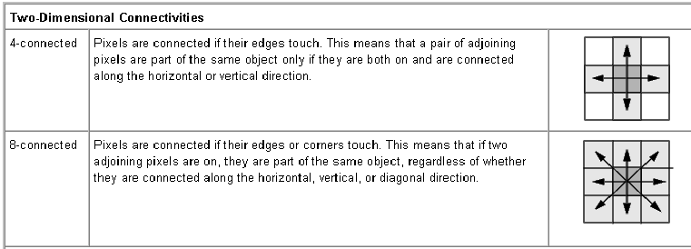
Figure 2.2 Pixel connectivity
A digital path (or curve) from pixel ( p ) with coordinates (x, y) to pixel ( q ) with coordinates ( s , t ) is a sequence of distinct pixels with coordinates ( x0 , y0 ), ( x1 , y1 ), …. , ( xn , yn ) where ( x0 , y0 ) = ( x , y ), ( xn , yn ) = ( s , t ), and pixels ( xi , yi ) and ( xi-1, yi-1) are adjacent for 1 ≤ i ≤ n. In this case, n is the length of the path. If (x0, y0) = (xn, yn), the path is a closed path.
We can define 4-, 8-, or m-paths depending on the type of adjacency specified. For example, the paths shown in Fig 2.1(b) between the northeast and southeast points are 8-paths, and the path in Fig 2.1(c) is an m-path. Note the absence of ambiguity in the m-path.
Let S represent a subset of pixels in an image. Two pixels p and q are said to be connected in S if there exists a path between them consisting entirely of pixels in S. For any pixel p in S, the set of pixels that are connected to it in S is called a connected component of S. If it only has one connected component, then set S is called a connected set.
Let R be a subset of pixels in an image. We call R a region of the image if R is a connected set. The boundary (also called border or contour) of a region R is the set of pixels in the region that have one or more neighbors that are not in R. If R happens to be an entire image (which we recall is a rectangular set of pixels), then its boundary is defined as the set of pixels in the first and last rows and columns of the image. This extra definition is required because an image has no neighbors beyond its border. Normally, when we refer to a region, we are referring to a subset of an image, and any pixels in the boundary of the region that happen to coincide with the border of the image are included implicitly as part of the region boundary.
The concept of an edge is found frequently in discussion dealing with regions and boundaries. There is a key difference between these concepts, however. The boundary of a finite region forms a closed path and is thus a “global” concept. Edges are formed from pixels with derivative values that exceed a preset threshold. Thus, the idea of an edge is a “local” concept that is based on a measure of gray-level discontinuity at a point. It is possible to link edge points into edge segments, and some times these segments are linked in such a way that correspond to boundaries, but this is not always the case. Depending on the type of connectivity and edge operators used, the edge extracted from a binary region will be the same as the region boundary. This is intuitive. Conceptually it is helpful to think of edges as intensity discontinuities and boundaries as closed paths.